Newbie Guide to Convolutional Neural Network (CNN)
introduction
Convolutional neural networks: It sounds like a strange combination of biology and mathematics and a small amount of computer science, but these networks have created some of the most influential innovations in computer vision. In 2012, neural networks began to emerge. In that year, Alex Krizhevskyj competed in the ImageNet competition (ImageNet was considered to be the annual “Olympic†competition in the field of computer vision competition). The classification error record was reduced from 26% to 15%, which was a Amazing progress. Since then, many companies have begun to apply deep learning to their core services. For example, Facebook has applied neural networks to their automated tagging algorithms. Google has applied them to image searches. Amazon has used them. Applied to product recommendation services, Pinterest applies them to the personalized flow of information on the homepage. Instagram also applies deep learning to their image search architecture.

However, the most classic, or the most popular example of neural network usage is to use it in the image processing field. Referring to image processing, this article mainly introduces how to use convolutional neural networks for image classification.
Problem space
Image classification is the task of sorting the input images (cats, dogs, etc.) or categorizing them into the categories that best describe the characteristics of the images. For humans, cognition is the first skill we learned after we were born, and it is also a very natural and relaxed skill for adults. We can quickly identify the environment and objects around us without hesitation. When we see a picture or observe the surrounding environment, most of the time we can immediately judge the scene and mark each object. You don't even need to deliberately observe it. These skills can quickly identify patterns, make inferences from our previous experience, and then apply them to different images or environments—these are where we differ from machines.
Input and output
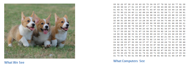
When the computer sees a picture (that is, enters a picture), what it sees is a series of pixel values. Based on the resolution and size of the picture, the computer will see a 32 x 32 x 3 digital array (3 refers to the RGB-color value). Let's take a look at this. Suppose we have a 480 x 480 JPG image with an array of 480 x 480 x 3. Each of these numbers can be taken from 0 to 255, which describes the pixel intensity at this point. Although these figures do not make any sense when we classify images, they are the only data the computer obtains when the images are input. The idea is that you specify the relevant data arrangement for the computer, which outputs the possibility that the image is a specific category (eg 80-cat, 15-dog, 05-bird, etc.).
What do we want the computer to do
Now that we understand the problem is in the input and output, let us consider how to solve this problem. What we want computers to do is to distinguish the different categories in all given images. It can find the characteristics of "dogs are dogs" or "cats are cats." This is the process of cognitive recognition in the subconscious mind of our mind. When we see a picture of a dog, we can classify it because the image has obvious features such as claws or four legs. In a similar manner, computers can perform image classification tasks by finding low-level features such as edges and curves, and then applying a series of convolutional layers to create a more abstract concept. This is a general overview of the convolutional neural network application. Next we will discuss the following details.
Biological connection
First of all, we need to use a bit of background knowledge. When you first hear the term convolutional neural network, you may think that this is not related to neuroscience or biology. Congratulations, guess right. The convolutional neural network is indeed inspired by the biological visual cortex. The cells in the tiny area of ​​the visual cortex are very sensitive to the field of view in a specific area.
In 1962, Hubel and Wiesel discovered that some neurons in the brain responded only to edges in certain directions. For example, some neurons respond when exposed to vertical edges or some horizontal or diagonal edges. Hubel and Wiesel discovered that all of these neurons are built into a columnar structure that enables them to produce visual perception. The idea that certain members of the system can accomplish specific tasks (neural cells look for specific features in the visual cortex) can also be well applied to machine learning, which is also the basis of convolutional neural networks.
Structure
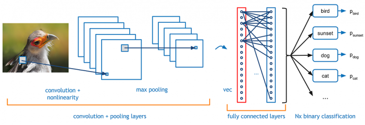
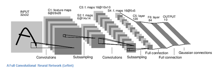
A more detailed introduction to the warped neural network is to pass the picture through a series of convolutions, non-linearities, pools (samples), full connected layers, and then get an output. As we said earlier, the output is the probability of a class or an image class. Now, the hard part is understanding the tasks of each layer.
First level - Mathematics
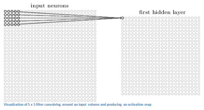
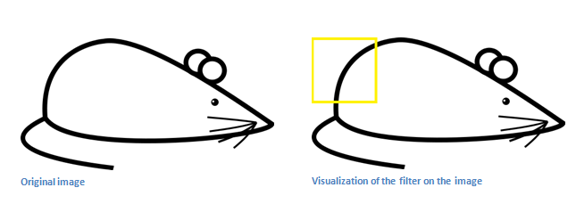
The first layer of a convolutional neural network is a convolutional layer. The first thing is that you have to remember what the input of the curl layer is. As we mentioned before, the input is a 32×32×3 series of pixel values. The best way to explain the convolution layer is to imagine that a flashlight is illuminating at the upper left of the image, assuming that the area illuminated by the flashlight is a 5 x 5 range. Then imagine the flashlight slides in each area of ​​the input image. In machine learning terminology, the flashlight is called a filter (sometimes called a neuron or core) and the area it illuminates is called the receiving field. This filter is also a series of data (these data are called weights or parameters). It must be mentioned that the depth of this filter must be the same as the input depth (this guarantees that mathematics works), so the size of this filter is 5 × 5 × 3. Now, let us first take the first position filter as an example. Since the filter is sliding or convolved on the input image, it is multiplied by the pixel value of the filter's original image (aka multiplication of the calculated element) and these multiplications are all added (mathematically, this Will be 75 multiplication sums). So now you have a number. Remember that this number is only representative when the filter is in the upper left corner of the image, and now we repeat this process at each position. (The next step is to move the filter to 1 unit on the right and then 1 unit to the right, etc.). A unique number will be generated on each input layer. Sliding the filter to all positions, you will find that the rest is a 28 × 28 × 1 series of numbers, we call it the activation map or feature map. The reason you get a 28×28 array is that there are 784 different locations. A 5×5 filter can fit a 32×32 input image. This group of 784 numbers can be mapped to a 28×28 array.
Currently we use two 5 x 5 x 3 filters. Our output will be 28 x 28 x 2. By using more filters, we can better maintain the space size. On a mathematical level, these are tasks that are performed in a convolutional layer.
First level - higher order
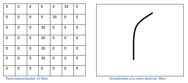
Let's talk about the task of this convolution layer from a high-level perspective. Each of these filters can be considered as a feature identifier. When I say features, I'm talking about straight edges, simple colors, and curves. Think about it, all images have the same simplest features. Our first filter is 7×7×3 and it is a curve detector. (In this section let us ignore the fact that the filter is 3 units deep and only considers the depth of the top filter and the image.) As a curve detector, the filter will have a higher value and a curved shape The pixel structure (remembering about these filters, we consider only numbers).
Now, let's go back to the math visualization section. When we have this kind of filter in the upper left corner of the input, it calculates the product between the filter and pixel values ​​in which region. Now let's take an image we want to classify as an example and put our filter in the top left corner.
Remember, what we need to do is use the original pixel value in the image to do the product in the filter.
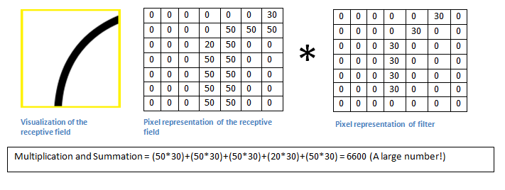
Basically in the input image, if there is a shape that is similar to the representative curve of such a filter, then all multiplications together add up to larger values! Let us now see what happens when we move our filter.
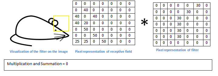
The detection value is actually much lower! This is because there is no partial response curve detection filter in the image. Remember that the output of this convolutional layer is an activation map. Therefore, in the simple case of convolution of a filter (if the filter is a curve detector), the activation graph will show that most of the curve area may be in the picture. In this example, the value at the top left of our 28×28×1 activation graph will be 6600. This high value means that it is likely that there is a curve in the input that caused the filter to activate. Since there is nothing to make the filter active at the input (or more simply, there is no curve for the original image in the area), its value at the top right of our activation graph will be 0. Remember, this is just a filter. This filter will detect the outward and right curve of the line, and we can have other filter lines left or right to the edge of the filter. The more filters there are, the deeper the activation map, and the more information we get from the input.
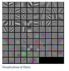
Statement: The filters described in this section are simplified and their main purpose is to describe the mathematical process in a convolution process. In the figure below you can see some actual examples of filters on the first convolutional layer in the trained network. However, the main argument is still the same.
Further in-depth network
Now show a traditional convolutional neural network structure, and there are other layers interspersed between these layers. It is strongly recommended that interested readers understand their function and role, but generally speaking, the non-linearity and size retention they provide can help increase the robustness of the network while also controlling overfitting. A classic convolutional neural network architecture looks like this:

However, the last layer is very important, but we will mention it later. Let's take a step back and review what we are currently talking about. We talked about the first convolutional filter designed to detect. They detected low-level features such as edges and curves. As you might imagine, in order to predict the type of image, we need neural networks to recognize higher-order features such as hands, paws, and ears. Let us consider what the output of the network is after going through the first layer of the convolution, which will be a 28 x 28 x 3 volume (assuming we use three 5 x 5 x 3 filters). When passing through another convolution layer, the first output of the convolution layer becomes the input of the second convolution layer, which is difficult to visualize. When we talk about the first layer, we only input the original image. However, when we talk about the second convolutional layer, the input is the result activation map (S) of the first layer. Therefore, the input of each layer basically describes the position of certain low-level features in the original image. Now when you apply a set of filters (via the second convolutional layer), the output will be activated and represent higher-order features. The type of these features may be a semicircle (a combination of curves and straight edges) or a square (a combination of several straight edges). When more convolutional layers are through the network, maps can be activated to represent more and more complex features. At the end of the neural network, there may be some activated filters that indicate when they see handwriting or pink objects in the image. Another interesting thing is that when you explore deeper in the network, filters start to have more and more acceptance fields, which means that they can receive information from a larger area or more of the original input.
Fully connected layer
Now we can detect these higher-order features, and the icing on the cake is to connect a fully connected layer at the end of the neural network. This layer basically takes an input amount (whether the output is a convolution or ReLU or a pool layer) and outputs an N-dimensional vector that is a program-selected category, as shown in the following figure. This fully-connected layer works by looking at the output of the previous layer (the activation graph that represents higher-order features) and determining which features are most relevant to a particular class. For example if the program predicts that some images are a dog, it will have a high value in the activation map, representing high-level features such as a paw or 4 legs. Similarly, if the program is to predict the function of some images as birds, it will have high-order values ​​in the activation graph, which represent higher-order features such as wings or beaks.
Training process
Training engineering as part of the neural network was deliberately not mentioned before because it may be the most important part. You may encounter many problems when reading, for example, how does the filter in the first convolutional layer know to look for edges and curves? How does the fully connected layer know where the activation map is? How do each layer's filter know what value it has? The way the computer can adjust its filtering value (or weight) is through a training process called back propagation .
Before we introduce back propagation, we must first review what we need to know about the operation of neural networks. At the moment we were born, our thoughts were brand new. We do not know what cats and birds are. Similarly, before the convolutional neural network begins, the values ​​of the weights or filters are random, the filters do not know to look for edges and curves, and the higher-order layer filters do not know to find paws and rakes. However, when we were slightly older, our parents and teachers showed us different pictures and images and gave us a corresponding label. The idea of ​​labeling images is both a training process for convolutional neural networks (CNNs). Before we talk about it, let us introduce a little. We have a training set. There are images of thousands of dogs, cats, and birds. Each image has a label that corresponds to what animal it is.
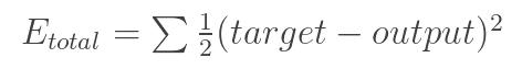
Back propagation can be divided into four different parts: forward propagation, loss calculation, back propagation, and weight update . In the process of propagation before, you need an array of numbers of training images of 32 × 32 × 3, and passed through the entire network. In our first training example, all weights or filter values ​​were randomly initialized and the output might be something like [.1.1.1.1.1.1.1.1.1.1.1.1] Basically, it is an output that cannot give priority to any number. The current weight of the network is unable to find those low-level functions, and therefore cannot make any reasonable conclusions about the classification possibilities. This is part of the loss calculation in reverse propagation. We are now using training data. This data has an image and a tag. For example, if the first input training image is a 3, the label of the image will be [0 0 1 0 0 0 0 0 ]. Loss calculations can be defined in many different ways, but it is common to square the MSE (mean squared deviation) — 1â„2 times (actual prediction).
Assuming that the variable L is equal to this value, as you might imagine, the loss will be very high for the first set of training images. Now let's think more intuitively. We want to get a point forecast tag (output of ConvNet) as training the same training tag (which means our network prediction is correct). To achieve this, we must minimize my loss. Visualization is only an optimization problem in calculus, and we need to find out which input is the weight (or weight in our example) that most directly leads to the loss (or error) of the network.

This is a mathematical equivalent of dL/DW, where W is the weight of a particular layer. Now what we need to do through the network is to perform a back-propagation process, detect which weight loss is greatest, and find ways to adjust them to reduce losses. Once we have finished this calculation process, we can go to the last step - updating the weights . The weights of all the filters are updated so that they change in the gradient direction.

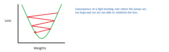
The learning rate is a parameter chosen by the programmer. A high learning rate means that more steps are in the weight update section, so it may take less time for the best weight to converge on the model. However, the high learning rate may lead to crossing over and not being precise enough to reach the best point.
The process of forward propagation, loss calculation, back propagation, and parameter update is also called an epoch. The process repeats this process for each fixed number of epochs, each training image. After the parameters were updated in the last training example, the network should be trained well and the weight of each layer should be adjusted correctly.
test
Finally, we want to test whether our convolutional neural network works, pass different pictures and tag sets through the convolutional neural network, compare the output results with the actual values, and test whether it works normally.
How the industry uses convolutional neural networks
Data, data, data. Given more training data for a convolutional neural network, more training iterations can be done, more weight updates can be achieved, and neural networks can be better adjusted. Facebook (and Instagram) can use all the current photos of hundreds of millions of users, Pinterest can use the 50 billion information on its website, Google can use search data, Amazon can use millions of products every day to buy data.
Now that you know how they use these magic, if you are interested, you can try it yourself.
PS : This article was compiled by Lei Feng Network (search “Lei Feng Network†public number) and it was compiled without permission.
Via Adit Deshpande