Real-time heuristic search: first result
Joint compilation: Zhang Min, Chen Jun
SummaryExisting heuristic search algorithms cannot take action before finding a complete solution, so they are not suitable for real-time applications. Therefore, we propose a special case of minimax lookahead search to deal with this problem. We also propose an algorithm similar to α-β pruning that can significantly improve the efficiency of the algorithm. In addition, we have proposed a new algorithm called Real-Time-A that can be used when the action must be performed, not just simulated. Finally, we examined the nature of the trade-off between computing and execution costs.
1 IntroductionHeuristic search is a fundamental problem solving method in the field of artificial intelligence. For most AI problems, the sequence of steps required for the solution may not be known a priori, but it must be decided by a system trial and error to explore alternative methods. All of these requirements construct a search problem—a series of states, a series of states that map to state operators, an initial state, and a series of target states. The typical problem with this task is to find one of the cheapest operators to map the initial state to the target state. The use of heuristic evaluation functions (generally without sacrificing the optimal solution) greatly reduces the complexity of the search algorithm. The heuristic function is relatively more affordable when calculating and evaluating the expenditure of the most affordable method from the given state to the target state.
A common example in the literary world of search problems is Eight Puzzle and its relatively large Fifteen Puzzle. Eight Puzzle consists of a 3x3 sequence box containing 8 numbered pieces and an empty position called 'blank'. The legal operator slides the pieces horizontally or vertically from adjacent positions. Its task is to rearrange the pieces to the desired setting in a random initial state. This problem has a common heuristic function called the Manhattan Distance. It is calculated in a counted manner. For each piece that is no longer at its target position, the number of moves along the grid is far away from it. The target position, and the total value of all pieces, does not include blanks.
A real-time example such as auto-navigation of network paths, or an arbitrary terrain from an initial position to the desired target position. This is a typical problem of finding the shortest path between the target and the initial position. A typical heuristic evaluation function for this problem is the spatial straight line from the given position to the target position.
Existing algorithmsThe most famous heuristic search algorithm is A. A is the calculation of which point f(n) is the best preferred optimal search algorithm, g(n) is the actual total expenditure for searching for this point, and h(n) is the evaluation expenditure for searching for the point solution. When a heuristic function can be adopted, A has a characteristic that it can always find the optimal solution to the problem. For example, the actual expenditure of the solution will never be overestimated.
Iterative-Deepening-A (IDA) is a modified version of A that reduces the spatial complexity from exponential to linear practice. IDA performed a series of depth-first searches. When the boundary point's expenditure exceeds the termination threshold, its branches are truncated, f(n) = g(n) + h(n). This threshold begins with a heuristic evaluation of the initial state and increases each iteration to a minimum (exceeding the original threshold). IDA has the same features as A in terms of optimal solution, and extends the point of the same instance, further, like A in an index tree, but it uses only linear space.
The common disadvantage of A and IDA is that they spend a lot of time operating in practice. This is the unavoidable expenditure for obtaining the optimal solution. As noted by Simon, however, although the optimal solution is relatively rare, the solution that is close to optimal or "satisfactory" for most real-time problems can usually be fully accepted.
There is also a common disadvantage between related A and IDA: they must search for all solutions before proceeding with the first step. The reason is that until the entire solution is found and it proves to be at least as good as other solutions, it is optimal to keep the first step. Therefore, A and IDA are completed in the planning or simulation phase before the first step in the implementation of the resulting solution in the real world. This greatly limits the application of these algorithms to real-time applications.
Real-time problemIn this section, we show several very important characteristics of real-time problems that must be considered in any real-time heuristic search algorithm.
The first characteristic is that problem solvers must face a limited range of practical problems. This is mainly caused by the limitation of calculation or information. For example, since the combination of the Fifteen Puzzle is soaring, when the DEC20 uses the Manhattan Distance IDA algorithm, the average time spent on each question is 5 hours. A bit of a problem on a large scale will not be solved. To prevent the negative effects of full-detail mapping, the search range (iteration, in this case) depends on the restriction of the information—how far the visual can be seen. Despite precise mapping, the level of detail is still limited. This leads to a "fuzzy horizon," where the level of detail of the terrain knowledge is a decreasing function to the distance of the problem solver.
A related feature is that in real-time settings, actions must be taken before their final results are known. For example, when playing chess, it is required that the pieces must be moved to extend the search range of the direction selection.
The last and most important characteristic is that the expenditure of the action and the planned expenditure can be expressed in the same occurrence, causing a trade-off between the two. For example, if the goal of Fifteen Puzzle is to solve the problem in the shortest time while moving a minimum number, then we will quantify the time for actual physical movement compared to simulating movement in the machine, and then in principle we will find an algorithm by balancing The "think" time and the "action" time minimize the total time of solution.
4. Minimized lookahead searchIn this section, we show a simple algorithm for heuristic search of single-agent problems (including all the previous features included). This is equivalent to the two-player game minimax algorithm. This is not new, because the two-player game shares the real-time nature of the limited search range and takes action before the final result is known. First we assume that all operators have the same expenditure.
The algorithm searches forward from the current state to a fixed depth (depending on the computation or information available monomer information), and applies a heuristic to evaluate the function to the point of the search front. In a two-player game, the values ​​are maximally minimized into the tree, causing players to move alternately. In a single-agent setup, since the single agent controls all movements, the backup value for each point is the minimum value for its next point. Once the next-step backup value of the current state is determined, a separate optimal next move will be performed in that direction, and this process is repeated as such. The reason for not moving directly to the minimum of the front-end point is: follow the strategy of the minimum commitment. Under this scenario, after arranging the first step, the added information (from the extended search frontier) may be more likely to affect the second choice than the first search. In order to contrast with the minimax search, we call this algorithm a minimum search.
Note: In addition to staggered models, the search process for the two methods is completely different. Minimal look-ahead search is performed in a simulation model in which the assumed movement is not actually performed and simulation is performed only in the machine. After a complete look-ahead search, find the optimal move by the problem solver in the real world. Then perform another look-ahead search in the current state, and actual movement.
In many common situations, operators have disparate expenditures, and we must calculate the expenditures of the routes so far so that the remaining expenditures can be evaluated heuristically. To perform this calculation, we use the A-spending function f(n)=g(n)+(h). The algorithm then advances a fixed amount of movement and backs up the minimum value f of each frontier point. The alternative searches forward for a fixed amount of movement while searching forward for a fixed g(n) expenditure. We use the original algorithm under this scenario, that is, calculating the expenditure during the planning phase is a function of the number of movements rather than a function of actually performing the mobile expenditure.
In order to ensure termination, care must be taken to prevent the problem solver from actually walking an infinite loop of paths. This has been accomplished by maintaining the CLOSED table for these states (the problem solver's actual visited and moved state), and the OPEN stack from the initial state to the current path point. Moving to the CLOSED state is the result output, and then the OPEN stack is used for backward tracking until the move can be used for a new state. This conservative strategy prohibits the algorithm from destroying previous movements unless it encounters a dead end. This limit will be removed later.
5.Alpha Pruning AlgorithmIt is natural to ask this step whether each frontier point must be tested to find the minimum expenditure, or whether there is an alpha-beta pruning algorithm that allows the same Decision. If our algorithm only uses frontier point evaluation, then a simple anti-idea can determine that no such pruning algorithm exists because determining the minimum expenditure frontier point requires the detection of each point.
However, if we allow heuristic evaluation of internal points, and the expenditure function is a monotonous function, then the pruning in essence is feasible. If the payoff function f(n) does not decrement to the initial state, then it is a monotonic function. The monotonicity of f(n)=g(n)+h(n) is the same as h(n), or follows a triangle inequality that satisfies the properties of the most naturally occurring heuristic function, including the Manhattan Distance and the space line. Distance (air-line distance). In addition, if the heuristic function is permissible but not monotonous, then an admissible, monotonic function f(n) can obviously be built with the maximum value of its path.
A monotonic f-function allows us to apply a branch-and-bound method to greatly reduce the number of detection points without affecting the decision. Analogous to the α-β pruning algorithm, we call this algorithm the α pruning algorithm, as follows: During the spanning tree, it is kept at a variable α (which is the lowest value of f at all currently encountered points in the search range). The value of f is calculated when each internal point is generated, and the corresponding branch is cut off when the value of f is equal to α. The reason this can be done is because the function is monotonic and the value of the front point f can only be decremented from a point that is better or equal to the point of expenditure, and it cannot affect the movement because we only move to the leading edge point of the minimum value. When each front edge point is generated, the f-value is also calculated. If it is smaller than α, a smaller value is used instead of α, and a search is performed.
In the Fifteen Puzzle experiment using the Manhattan Distance evaluation function, the alpha pruning algorithm reduced the effective branching factor by far more than the square root of the brute-force branching factor (from 2.13 to 1.41). In the same number of calculations, its effect is better than twice the search range. For example, if the calculation source allows millions of points to be detected while moving, then the beta compression algorithm can search for a depth of 18 moves, while the alpha pruning algorithm allows for a search depth of nearly twice (40 steps).
In the alpha pruning algorithm, the efficiency of the alpha pruning algorithm can be improved by node ordring. The idea is to order the order of the f-values ​​for each internal point's inheritance point, hoping to find the minimum spending to find the frontier point earlier, and to cut the branch more quickly.
Although these two algorithms are developed separately, minimizing the alpha pruning algorithm is very similar to a single iteration of iterative-deepening-A. The only difference is that in the alpha pruning algorithm, the discontinuity threshold is dynamically determined and adjusted by the minimum of the leading edge point, rather than iteratively pre-fixed and set in the IDA previously.
6. Real-time ASo far we have imagined that once an act is executed unless it encounters a dead end, it will not be reversed. - The main motivation is to stop the problem solver from going into an endless loop. The problem we are solving now is: how can it be useful to return, rather than die while returning, while still invalidating the loop anyway. The basic idea is very simple. When evaluating the solution from the state (plus returned expenditures) to the state (less than the estimated expenditure moving forward from the current state), it should return to its original state. Real-Time-A is a very effective algorithm for implementing this basic idea.
The minimum lookahead algorithm is an algorithm that controls the search simulation phase, and RTA is an algorithm that controls the search execution phase. Therefore, it is independent of the selected simulation algorithm. Simply put, we assume that the minimum look-ahead depth is encapsulated within the calculation h(n), and therefore, becomes simpler, more accurate, and calculates h(n) more expensively.
In RTA, the advantage of point n is that f(n) = g(n) + h(n), as in A. However, unlike A, the understanding of g(n) in RTA is the distance from point n to the current state of the problem solver, rather than the original initial state. RTA is just the best first search given a slightly different payoff function. In principle, it can be achieved by storing the h-value OPEN table of all previously visited points, and each move will update the g value of all states on the OPEN to accurately reflect their actual distance to the new current state. Then in each move cycle, the problem solver selects the next state by the minimum value of g+h, moves to it, and updates the g value of all states on OPEN again.
The disadvantages of this simple implementation are: 1) The size of the time in the OPEN list is linearly shifted. 2) It is not very clear how to update the value of g, 3) It is not clear how to select the path of the next target node from OPEN. Interestingly, these problems can be solved by using only the local information in the graph to move at a constant time. The idea is as follows: from the given current state, neighboring states can be generated, heuristics are enhanced by forward search (this applies to all cases), and then the cost of each neighboring edge increases by this value, resulting in the current state of each The f-value of a neighborhood. The point with a very small f-value is selected from the new current state and the movement (the state that has already been executed). At the same time, the next f-value is stored in the previous current state.
This represents the cost of solving such problems by returning to the original state. Next, new neighbors in the new state are generated, and their h-values ​​are also calculated, and the edge costs of all neighbors in the new state, including the previous state, are added to the h-value, resulting in all neighbors. State A series of f-values. Again, the node with the smallest value is removed and the second best node value is stored in the h value of the old state.
Note that RTA does not need to separate the OPEN and CLOSED lists. A single list of previously evaluated node values ​​is sufficient. The scale of the table is linear with the number of moves, because the feedforward search will only preserve the root node value. And the running time also has a linear relationship with the number of steps. The reason is that despite the exponential growth of the time required for the feed-forward study and the depth of the study, the study depth will be constrained by constants.
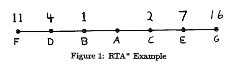
Interestingly enough, people can create an example to prove that RTA traces any number of times in the same field. For example, in the simplest strighthne graph in Figure 1, the initial state is node a, all edges have a global value, and the value under each node represents a heuristic evaluation of these nodes. Since feedforward will only make the example more complicated, we will assume that there is no feed forward energy to calculate the value of h. And at the beginning of node a, f(b)=g(b)+h(b)=1+1=2, but f(c)=g(c)+h(c)=1+2=3. Therefore, the problem solver moves to node b and leaves node a in the information state of h(a)=3. Next, node d evaluates f(d)=g(d)+h(d)=1+4=5, so node a becomes f(a)=g(a)+h (a)=1+3=4 results. So the problem solver moves back to node a, and h(b) = 5 after node b. Based on this, f(b)=g(b)+h(b)=1+5=6, and f(c)=g(c)+h(c)=1+2=3, resulting in problem solving The program has moved to node c again so that h(a) = 6 after node a. The reader can't wait to continue the example to witness the problem solver continually making a round trip until it reaches the goal. The principle is not that it is an infinite ring, but that when it changes its direction, it can go one step further than before and it can gather more information about space. This seemingly unreasonable behavior is caused by rational behavior within the limits of limited exploration and pathology.
Unfortunately, RTA's traceability cannot be used as a Fifteen Puzzle and Manhattan Distance evaluation function. This is because the Manhattan Distance changes only once in one move, and this causes the RTA to terminate once it is traced.
In addition to the efficiency of the algorithm, the length of the solution resulting from the minimum feedforward search is also the focus of attention. The most normal expectation is that the depth will increase as the length of resolution is reduced. Using Manhattan Distance in experiments with the Fifteen Puzzle, the results show that expectations are correct, but not consistent.
One thousand original settlements of Fifteen Puzzle are randomly generated. For each original state, the minimum value of the alpha pruning algorithm is between 1 and 30 steps deep in the search. In order to find a solution, it will move continuously, so it is possible to reach 1,000 steps. Therefore, in order to prevent the number of steps from being too long, all the number of result steps will be recorded. Figure 2 shows the average length of the solution and the depth of the search limit in all over 1,000 steps. The bottom line shows 53 average optimal steps in 100 different original states. The length of the optimal solution is calculated using IDA and takes a few weeks of CPU time to resolve hundreds of original conditions.
The general shape of the curve confirms the initial assumption that increasing the search range limit can reduce the cost of solving the calculation. At a depth of 25, the length of the average solution is only one factor better than the average length of the optimal solution. This result is achieved by searching only 6000 nodes at each step, or only searching 6000,000 nodes for the entire solution. This process requires only one minute of CPU runtime on the Hewlett-Packard HP-9000 workstation.
However, at depths of 3, 10, or 11, increased search limits can cause a slight increase in the length of the solution. This phenomenon was first discovered in games with two players and Pathology named by Dana Nau. He found that in some games, search depth was increased but the game results were still poor. Until, in the real game path observation.
Although the impact of the route will be relatively small when a large number of problems are involved, the impact on the individual issues is still very important. In most cases, increasing the depth of search in one step will increase the length of the solution by hundreds of steps.
In order to better understand this phenomenon, we test the "determination quality", which corresponds to the quality of the solution. The difference between them is that a solution involves a large number of individual decisions. The quality of the solution is determined by the length of the solution, and the quality of the decision is determined by the time taken to choose the optimal step. Since you must know the optimal step in a state to determine the quality of the decision, choose the smaller, or docile, Eight Puzzle and use the same Manhattan Distance evaluation function.
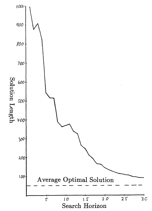
Figure 2: Search Limit vs. Resolution Length
In this case, thousands of primitive states are randomly generated. We will not explore the entire solution because it is generated by the minimal algorithm; we only consider the first step in the original state. With different search limits and different initial conditions, the decision time for the first step of the first step is recorded. Search limits range from one step to the number of steps below the optimal choice. Figure 3 shows the error rate and search limitations. As the search limit increases, the optimal number of steps increases. Therefore, pathology does not appear to determine quality.
If the quality of the decision can increase with the depth of the search, why is the quality of the solution so erratic? One of the reasons is that when the odds of making mistakes increase, the cost of individual errors will increase in terms of overall cost. This is particularly evident when retrospective only occurs when a dead end is encountered.

Figure 3: Search Limit vs. Decision Quality
Another source of error is that the nodes are in alternatives. When the information is uncertain, it is necessary to determine the movement, but the connection should not be destroyed at will. More generally, when processing based on inaccurate heuristic evaluations, the accuracy of the two values ​​closer to the function should not be considered a virtual connection, and the processing for this should also be seen as indistinguishable. . To solve this problem, connections and virtual connections must be recognized at first glance. This also means that the alpha pruning algorithm must change when the value exceeds the best result originally affected by the error factor. This will lead to an increase of the resulting nodes.
Once the node is confirmed, it must be destroyed. The ideal method is to implement a deeper secondary search among candidate solutions until the connection collapses. However, this second search also has a deep limit. If the secondary search reaches the depth limit and the connection does not collapse, the virtual connection will disintegrate at a lower cost.
8. Calculation & ExecutionThe heuristic evaluation function is examined using a feed-forward search. According to the depth of search, a more accurate heuristic function can produce a series of heuristic functions. This series of functions has different computational complexity and accuracy, but generally more expensive functions are even more accurate.
Which evaluation function is chosen to balance the search cost and determine the cost. The minimization of time depends on the associated computational costs and decisions, but a reasonable model is that each one is linearly related to each other. To put it another way, if we assume that the cost of using an arithmetic operation in practice is the sum of all simulations.
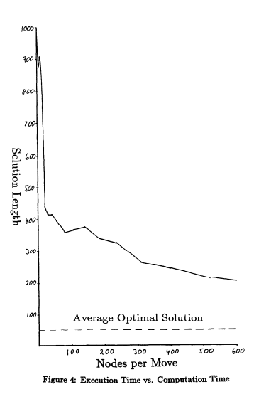
Figure 4 shows the same data as Figure 2, but the horizontal axis is linear with the number of nodes generated at each step, which is also strongly related to the depth of the search. This graph shows that calculations are performed to a certain degree in the first instance, for example, a small amount of computational increase will bring about a large amount of decision-making cost reduction. However, when it comes to reducing turning points, the decision to reduce costs requires a lot of calculations. This effect may also be greater than the original, because the length decision process requires any one hundred steps. The relationship between different calculation costs and execution changes the relationship between the two axes, but does not change the basic shape of the basic curve L.
9. ConclusionThe existing single-agent heuristics cannot be used in practice because the cost of calculation cannot be predicted until the calculation is stopped. Minimized feedforward search is the best solution to this type of problem. In addition, the alpha pruning algorithm can improve the effectiveness of the algorithm, but it does not affect the execution of the decision. In addition, the real-time alpha algorithm solves the problem of abandoning the current algorithm when it meets more promising algorithms. A large number of simulations show that increasing the search depth will generally improve the quality of the decision, but the opposite situation is normal. In order to avoid a virtual connection having a decisive influence on the quality, additional algorithms are also necessary. Finally, the feedforward algorithm can be seen as producing a series of searches with different accuracy and computational difficulty. The relationship between the quality of the decision and the cost of calculation is initially mutually supportive, but at the same time it will quickly reach a point of diminishing returns.
Via: the original site of the paper
Comments from Associate Professor Li Yanjie of Harbin Institute of Technology: As the traditional single-agent heuristic search algorithms, such as the A algorithm, have a relatively large amount of calculations and need to be searched after the final result is executed, they are not suitable for occasions with high real-time requirements. Therefore, this paper studies the problem of real-time heuristic search. In this paper, we use the miniminimum look-ahead search to avoid the problems mentioned above in the traditional heuristic search, and use the alpha pruning method to improve the efficiency of the algorithm. The combination of the two ideas is actually an adaptive version of the IDA algorithm. That is, the pruning threshold is dynamically adjusted adaptively as the search node changes, rather than being statically preset as in the IDA algorithm. In addition, a real-time A algorithm is presented in this paper to implement the conversion of the current search path to a better path.
PS : This article was compiled by Lei Feng Network (search "Lei Feng Network (search "Lei Feng Network" public number attention " "public number attention"), without permission, refused to reprint!